Tour through 107 German Cities Shortest Tours: The Travling Salesman Problem Technische Universität München

Shortest round trips

Welcome to the TSP game!

This website is about the so-called "Traveling Salesman Problem".

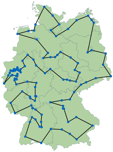
It deals with the question, how to plan a complete round trip through a certain number of cities to obtain the shortest tour possible. This question can be answered quite easily for four cities. However, it gets complicated when the number of cities is increased. There exist for example 181.440 different tours through just ten cities.

How can one find the shortest tour on twenty or even more cities?

For this reason, various algorithms have been invented, which try to solve the Traveling Salesman Problem as fast as possible.

And now it is your turn!

Create a new game in the next tab and try to find a shortest tour yourself! Afterwards, you may have a look at the solution and the calculation steps of the applied algorithms.

Have fun!

What would you like to do first?

Tour durch 107 Städte Deutschlands

New Game

Map:


Metrics:

Repeat game

Game Code:
Error

    On this page you can create a new game!

    Choose a map and the number of cities, that have to be visited. If your choice is the "Grid", you may choose one out of three different metrics. It determines the way distances are calculated.
    Euclidean metrics Euklidsche Metrik
    (x1-x2)2 + (y1-y2)2 
    One metrics Euklidsche Metrik
    |x1-x2|+|y1-y2|
    Maximum metrics Euklidsche Metrik
    max{|x1-x2|,|y1-y2|}
    Ihr Browser unterst¨tzt kein HTML5 Canvas. Bitte verwenden Sie einen modernen Browser, z.B.Mozilla Firefox

    Length of your tour:

    0 km

    Find your tour!

    Draw your round trip!
    Try to find the shortest possible, but do not forget to visit all of the cities.
    By right or double click you can delete an already drawn path. Filled cities have already been visited and left again.

    See the solution!

    As soon as you have visited all of the cities, you can get the optimal tour displayed here and compare it to your own solution. If you would like to see the solution instantly, just press 'Optimal tour' in the tab bar.
    You do not visit all nodes!
    Your tour contains subtours!

    Repeat the current game!

    In order to play the current game again later, you can get the GameCode displayed here and type it in under 'Repeat game' while creating a game.
    Show GameCode...

    Test your logistic skills and draw the shortest round trip you can find.

    Do not forget to visit every city exactly once!

    By changing the tab, the drawing mode will be terminated.

    There is no way back to the "Play game" tab.

    Ihr Browser unterstützt kein HTML5 Canvas. Bitte verwenden Sie einen modernen Browser, z.B.Mozilla Firefox

    Length of the optimal tour:

    0 km

    Length of your tour:

    0 km

    Calculation time:

    0 ms

    Congratulations! Your tour is optimal.

    Too bad! Unfortunately, your tour is not optimal.

    Too bad! Unfortunately, your tour does not visit all nodes.

    Too bad! Unfortunately, your tour contains subtours.

    How has the solution been calculated?

    By clicking the button you will get further information regarding the functional principles of the applied algorithms, which contributed to the solution.
    Alternatively, you can directly get the calculation steps displayed, which led to this round trip.
    Show GameCode...

    Congratulations! Your tour is optimal.

    Too bad! Unfortunately, your tour is not optimal.

    Too bad! Unfortunately, your tour does not visit all nodes.

    Too bad! Unfortunately, your tour contains subtours.

    Optimal tour:
    Your tour:

    In this tab you may have a look at the optimal tour and the corresponding calculation steps.

    In the Description of the algorithm you may find more details on the applied algorithms of the different steps.

    On this page you may have a look at how the different algorithms work. Feel free to click on the name of the algorithm that you are interested in knowing more about.

    Graphs and algorithms

    Points on the map of the game represent cities. A line between two cities represents the shortest connection between them.
    In so-called graph theory, points are called 'nodes' and lines are referred to as 'edges'. A collection of nodes and edges is called 'graph'.
    Speaking about algorithms regarding the Traveling Salesman Problem, one distinguishes between two basic types:
    • 'Heuristics', which find a round trip, but do not indicate its optimality in relation to an optimal solution. Its length is always larger than the length of an optimal tour. It is than called 'upper bound'.
    • "Exact solver", which converge to an optimal round trip slowly. Found paths are never longer than an optimal solution. Therefore, their length is called 'lower bound'. Their result is rarely a round trip through all nodes.
    One knows subsequently, that the length of a shortest round trip must be between these two bounds. The better the used algorithms are, the smaller is the difference between both bounds and the more precise is the found length of an optimal tour.

    Nearest neighbour algorithm

    The Nearest Neighbor Algorithm is probably the most intuitive of all TSP algorithms.
    First, one chooses a node to start from.
    As the algorithm's name already tells, one goes to the node being the closest to the current node. Naturally, one must always head at nodes, which have not been visited throughout the tour.
    This step is repeated until no more node is available. Afterwards, one returns to the starting node.
    Although it seems that one would always obtain a shortest round trip by using this method, this is not the case. In the 'calculation steps' tab you can easily see, that such a tour is rarely optimal. There, the Nearest Neighbor Algorithm is applied to a graph at first.

    Multiple fragment algorithm

    The Multiple Fragment Algorithm puts the round trip together by inserting 'multiple fragments', like a puzzle. Therefore, all edges are sorted by their length in ascending order. Afterwards, one adds one edge after another to graph, starting with the shortest edge.
    When doing this, two constraints have to be fulfilled:
    • There are no more than two incident edges allowed for each node.
    • No circles are allowed.
    This method always leads to a round trip.

    Lagrangian relaxation

    The Lagrange relaxation used on this page expands the set of possible solutions by the so-called 'minimal One-trees'. A One-tree is a path, that visits all nodes exactly once and contains exactly one circle after adding an additional edge. It is called 'minimal', if one only chooses the shortest edges. Afterwards, the length of all edges will be manipulated in a way that the result of the next calculation step ist different to the found One-tree of the current step.
    It works as follows:
    • Remove one node from the graph.
    • Add edges between the remaining nodes in ascending order, like in the Multiple Fragment algorithm. There may be more than two edges incident to one node. However, circles are not allowed.
    • Now add the removed node together with its two shortest incident edges to the graph. If a round trip is obtained, stop. There is no shorter round trip. Otherwise, one continues as follows.
    • The aim is to have exactly two edges incident to one node. Therefore, find out by which number the number of incident edges differs from 2. Say four edges are incident to a node, then the result is 2. One incident edge leads to -1. Add the result to the length of all incident edges.
    • Return to the first step.
    Since this method may take a long time until it finds an optimal solution, it may be a good idea to set a criterion, when to cancel the calculation.

    Branch and Bound

    The Branch and bound algorithm is very closely related to the Lagrange relaxation. If the latter could not find a solution, one makes the set of possible solutions smaller and afterwards runs the Lagrange relaxation on this new set again.
    At first, one chooses a node that was incident with three edges in the last solution. Afterwards, one creates three new problems, which are tried to be solved by using the Lagrange relaxation.
    Therefore, edges are either 'forced' or 'permitted' in the next solution. All other edges are called 'free'. These three problems are set according to following rules. Two of the incident edges shall therefore be called e and f:
    • e and f are forced edges. All other edges are permitted.
    • e is forced and f permitted. Edges that have been free before this step will stay free.
    • e is permitted. All other edges stay free, if they have been before.
    It is important to know that these rules exclude each other. A result obtained by using the first, second or third rule cannot be obtained by using any of the other two rules.
    In addition, the current solution is also excluded from following results. Since one chose a node, which is incident to three nodes and the first rule forces exactly two incident edges, the number of incident edges changes subsequently. Since both of the other rules exclude one of the edges, that have been incident to the node before, it is shown that the current solution can not be obtained again.
    Ihr Browser unterstützt kein HTML5 Canvas. Bitte verwenden Sie einen modernen Browser, z.B.Mozilla Firefox

    Origins of the Traveling Salesman Problem

    The Traveling Salesman Problem deals with problem of finding a tour visiting a given set of cities (without visiting one twice) such that the total distance to be traveled is minimal.
    The first time that this problem was mentioned in the literature was in 1831 in a book of Voigt. Its titel is "Der Handlungsreisende wie er sein soll und was er zu thun hat, um Aufträge zu erhalten und eines glücklichen Erfolgs in seinen Geschäften gewiss zu sein. Von einem alten Voyageur." (approx. "The traveling salesman, what he has to be like and what he has to do to obtain orders and success in his business. From an old voyageur." in English). Of importance is an excerpt of the last pages:
    [...] By appropriate Choice and Planning of the tour one often can save that much time that we will offer some proposals. [...] The most important aspect is to visit as many places as possible, without visiting one twice. [...]
    Although these two sentences meet the problem description of the Traveling Salesman Problem in great length, the formal introduction of the problem into Mathematics is dated to an article of Karl Menger in the context of the Mathematical Colloquium in Vienna in 1930:
    We name the Delivery Boy Problem (because this question in praxis has to be solved by each delivery boy, as well as by lots of travelers) the task of, for a finite set of points with known pairwise distances, finding the shortest path visiting all points.
    Of course, this formulation does not completely coincide with the description of the Traveling Salesman Problem, as the shortest path instead of the shortest tour is required.
    Nonetheless, the problem made its way from Vienna to Hassler Whitney in 1931/1932, who presented it using todays name at the University of Princeton in 1934.

    The application

    The application presents some algorithms used to solve the Traveling Salesman Problem. Here, algorithms that can easily be visualized and explained in an understandable way were chosen. The development of these methods dates back quite some time, thus they obviously do not present the status quo of research for the Traveling Salesman Problem.

    Studying mathematics at the TUM

    Further graph algorithms are explained on the homepage of chair M9 of the TU München.
    Studying mathematics at the TU München answers all further questions concerning graph theory (as long as an answer is known).

    A last remark about this page's goal and citations

    Chair M9 of Technische Universität München does research in the fields of discrete mathematics, applied geometry and the optimization of mathematical problems. The problem and corresponding algorithms presented here are a famous example for the application of mathematics on an applied problem (and can be assigned to the field of combinatorial optimization). This page shall help the reader to recognize the application of mathematics to real life problems and to understand easy mathematical solution methods used. The algorithms presented were chosen according to understandability, they do not represent fields of research of the chair.

    To cite this page, please use the following information:

    There is no solution available.

    The calculation of the solution is still in progress. Please try again later.

    The calculation of the solution has been aborted. Please return to the Create game tab and start a new game.