Introduction
Create a graph
Run the algorithm
Description of the algorithm
Exercise 1
Exercise 2
More

What's the cheapest way from left to right?

Shortest paths and cheapest paths

In many applications one wants to obtain the shortest path from a to b. Depending on the context, the length of the path does not necessarily have to be the length in meter or miles: One can as well look at the cost or duration of a path – therefore looking for the cheapest path.

This applet presents the Bellman-Ford Algorithm, which calculates shortest paths even when cost can be negative.

What do you want to do first?

SVG Download

Legend

	Node
	Edge with weight 50

Legend

Which graph do you want to execute the algorithm on?

Start with an example graph:

Select

Modify it to your desire:

To create a node, make a double-click in the drawing area.
To create an edge, first click on the output node and then click on the destination node.
Right-clicking deletes edges and nodes.

Download the modified graph:

Download

Upload an existing graph:

occured when reading from file:

the contents:

What next?

SVG Download

Legend

	Starting node from where distances and shortest paths are computed.
	"Predecessor edge" that is used by the shortest path to the node.

Legend

Algorithm status

rewind fast forward

Explanation
Pseudocode

BEGIN

d(v[1]) ← 0

FOR j = 2,..,n DO

d(v[j]) ← ∞

FOR i = 1,..,(|V|-1) DO

FOR ALL (u,v) in E DO

d(v) ← min(d(v), d(u)+l(u,v))

FOR ALL (u,v) in E DO

IF d(v) > d(u) + l(u,v) DO

Message: "Negative Circle"

END

Variable status:

i	d(u)	d(v)	l(u,v)

Task is terminated if the tab is changed.

You can open another browser window for reading the description in parallel.

What's the cheapest way from left to right?

Shortest Paths

In many applications one wants to obtain the shortest path from a to b. Depending on the context, the length of the path does not necessarily have to be the length in meter: One can as well look at the cost of a path – both if we have to pay for using it – or if we receive some.

In general we speak of cost. Therefore one assigns cost to each part of the path – also called "edge".

Dijkstra's Algorithm computes shortest – or cheapest paths, if all cost are positive numbers. However, if one allows negative numbers, the algorithm will fail.

The Bellman-Ford Algorithm by contrast can also deal with negative cost.

These can for example occur when a taxi driver receives more money for a tour than he spends on fuel. If he does not transport somebody, his cost are positive.

Idea of the Algorithm

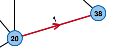
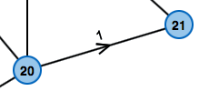
This edge is a short-cut:
We know that we have to pay 20 in order to go from the starting node to the left node. The path from the left to the right node has cost 1.
Therefore one can go from the starting node to the node on the right with a total cost of 21.

The Bellman-Ford Algorithm computes the cost of the cheapest paths from a starting node to all other nodes in the graph. Thus, he can also construct the paths afterwards.

The algorithm proceeds in an interactive manner, by beginning with a bad estimate of the cost and then improving it until the correct value is found.

The first estimate is:

The starting node has cost 0, as his distance to itself is obviously 0.
All other node have cost infinity, which is the worst estimate possible.

Afterwards, the algorithm checks every edge for the following condition: Are the cost of the source of the edge plus the cost for using the edge smaller than the cost of the edge's target?

If this is the case, we have found a short-cut: It is more profitable to use the edge which was just checked, than using the path used so far. Therefore the cost of the edge's target get updated: They are set to the cost of the source plus the cost for using the edge (compare example on the right).

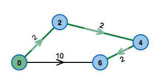
Looking at all edges of the graph and updating the cost of the nodes is called a phase. Unfortunately, it is not sufficient to look at all edges only once. After the first phase, the cost of all nodes for which the shortest path only uses one edge have been calculated correctly. After two phases all paths that use at most two edges have been computed correctly, and so on.

The green path from the starting node is the cheapest path. It uses 3 edges.

How many phases ware necessary? To answer this question, the observation that a shortest path has to use less edges than there are nodes in the graph. Thus, we need at most one phase less than the number of nodes in the graph. A shortest path that uses more edges than the number of nodes would visit some node twice and thus build a circle.

Construction of the shortest path

Each time when updating the cost of some node, the algorithm saves the edge that was used for the update as the predecessor of the node.

At the end of the algorithm, the shortest path to each node can be constructed by going backwards using the predecessor edges until the starting node is reached.

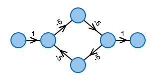
Circles with negative weight

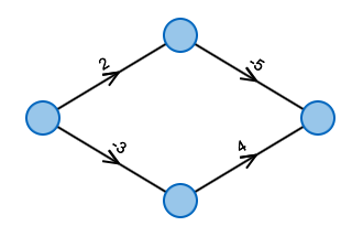
A cheapest path had to use this circle infinitely often. The cost would be reduced in each iteration.

If the graph contains a circle with a negative sum of edge weights – a Negative Circle, the algorithm probably will not find a cheapest path.

As can be seen in the example on the right, paths in this case can be infinitely cheap – one keeps on going through the circle.

This problem occurs if the negative circle can be reached from the starting node. Luckily, the algorithm can detect whether a negative circle exists. This is checked in the last step of the algorithm.

A negative circle can be reached if and only if after iterating all phases, one can still find a short-cut. Therefore, at the end the algorithm checks one more time for all edges whether the cost of the source node plus the cost of the edge are less than the cost of the target node. If this is the case for an edge, the message "Negative Circle found" is returned.

One can even find the negative circle with the help of the predecessor edges: One just goes back until one traversed a circle (that had negative weight).

What now?

Create a graph and play through the algorithm

Test your knowledge in the exercises

SVG Download

Legend

	Starting node from where distances and shortest paths are computed.
	"Predecessor edge" that is used by the shortest path to the node.

Legend

Test your knowledge: How does the algorithm decide?

rewind Forward: Next question

Explanation
Pseudocode

BEGIN

d(v[1]) ← 0

FOR j = 2,..,n DO

d(v[j]) ← ∞

FOR i = 1,..,(|V|-1) DO

FOR ALL (u,v) in E DO

d(v) ← min(d(v), d(u)+l(u,v))

FOR ALL (u,v) in E DO

IF d(v) > d(u) + l(u,v) DO

Message: "Negative Circle"

END

The task is terminated if the tab is changed.

You can open another browser window for reading the description in parallel.

SVG Download

Legend

	Starting node from where distances and shortest paths are computed.
	Edge that has already been selected.
	Edge that has been selected in the previous step.

Legend

What is the optimal ordering of the edges?

The Bellman-Ford Algorithm can compute all distances correctly in only one phase.

To do so, he has to look at the edges in the right sequence. This ordering is not easy to find – calculating it takes the same time as the Bellman-Ford Algorithm itself.

As one can see in the example: The ordering on the left in reasonable, after one phase the algorithm has correctly determined all distances. This is not the case on the right.

In this exercise you can test how many phases the algorithm needs for different sequences of the edges.

Task is terminated if the tab is changed.

You can open another browser window for reading the description in parallel.

What is the pseudocode of the algorithm?

Input: Weighted, undirected graph G=(V,E) with weight function l.
Output: A list {d(v[j]) : j = 1,..,n} containing the distances dist(v[1],v[j]) = d(v[j]),
         if there are no negative circles reachable from v[1]. 
         The message "Negative Circle" is shown, if a negative circle can be reached from v[1].


BEGIN
   d(v[1]) ← 0
   FOR j = 2,..,n DO
      d(v[j]) ← ∞
   FOR i = 1,..,(|V|-1) DO
      FOR ALL (u,v) in E DO
         d(v) ← min(d(v), d(u) + l(u,v))
   FOR ALL (u,v) in E DO
      IF d(v) > d(u) + l(u,v) DO
         Message: "Negative Circle"
END

How fast is the algorithm?

Speed of algorithms

The speed of an algorithm is the total number of individual steps which are performed during the execution.

These steps are for example:

Assignments – Set distance of a node to 20.
Comparisons – Is 20 greater than 23?
Comparison and assignment – If 20 is greater than 15, set variable n to 20
Simple Arithmetic Operations – What is 5 + 5?

Since it can be very difficult to count all individual steps, it is desirable to only count the approximate magnitude of the number of steps. This is also called the running time of an algorithm. Particularly, it is interesting to know the running time of an algorithm based on the size of the input (in this case the number of the vertices and the edges of the graph).

Running time of the Bellman-Ford Algorithm

We assume that the algorithm is run on a graph with n nodes and m edges.

At the beginning, the value ∞ is assigned to each node. We need n steps for that.

Then we do the n-1 phases of the algorithm – one phase less than the number of nodes. In each phase, all edges of the graph are checked, and the distance value of the target node may be changed. We can interpret this check and assignment of a new value as one step and therefore have m steps in each phase. In total all phases together require m · (n-1) steps.

Afterwards, the algorithm checks whether there is a negative circle, for which he looks at each edge once. Altogether he needs m steps for the check.

The total running time of the algorithm is of the magnitude m · n, as the n steps at the beginning and the m steps at the end can be neglected compared to the m · (n-1) steps for the phases.

How can one prove that the result is always correct?

A mathematical proof

In this section we will prove that the Bellman-Ford Algorithm always returns a correct result, if the graph does not contain negative circles that can be reached from the starting node.

The principle of induction

The proof is based on the principle of induction. We first prove that at the beginning of the first phase, the cost for at least one node have been calculated correctly. Then, we show that in each phase we improve the current estimates. At the end of each phase, we thus know the correct cost for more nodes than at the beginning of the phase. Additionally, we do not destroy any information in the respective phase – the estimates can only get better.

Finally, we conclude that we do not need as many phases as the number of nodes in order to compute the correct cost correctly.

After phase `i` the following holds:

The algorithm has – as an estimate – assigned to each node u maximally the length of the shortest path from the starting node to u that uses at most i edges (if such a path exists).

Let us have a look at this statement in detail for a node u at the end of phase i:

If no path from the starting node to u that uses at most i edges exists, we do not know anything.

If a path from the starting node to u using at most i edges exists, we know that the cost estimate for u is as high as the cost of the path or lower. The reason is the following: If we consider the path without its last edge, we yield a path using i-1 edges. The cost of the path's last node has been calculated correctly in the last phase. In this phase we have considered all edges, including the last part of the path. As we have updated the cost correctly when considering the last part of the path, the cost of the last node of the path (that is using i edges) correctly.

The number of phases needed is smaller than the number of nodes.

A path using at least as many edges as the number of nodes cannot be a shortest path if all circle have positive total weight. With each edge the path uses he "sees" another node (the target node of the edge). Additionally, we have to count the starting node the path saw without using another edge. If he uses as many edges as the number of nodes, it has seen at least one node twice or – to rephrase it – has used a circle. As we have assumed that all circles have positive weight, skipping the circle would have been shorter.

If there are circles with a total weight of 0, it simply is as expensive to use the circle than to not do it. In this case paths that use less edges than the number of nodes suffice as well.

Where can I find more information about graph algorithms?

Other graph algorithms are explained on the Website of Chair M9 of the TU München.

Furthermore there is an interesting book about shortest paths: Das Geheimnis des kürzesten Weges

Studying mathematics at the TU München answers all questions about graph theory (if an answer is known).

A last remark about this page's content, goal and citations

Chair M9 of Technische Universität München does research in the fields of discrete mathematics, applied geometry and the mathematical optimization of applied problems. The algorithms presented on the pages at hand are very basic examples for methods of discrete mathematics (the daily research conducted at the chair reaches far beyond that point). These pages shall provide pupils and students with the possibility to (better) understand and fully comprehend the algorithms, which are often of importance in daily life. Therefore, the presentation concentrates on the algorithms' ideas, and often explains them with just minimal or no mathematical notation at all.

Please be advised that the pages presented here have been created within the scope of student theses, supervised by Chair M9. The code and corresponding presentation could only be tested selectively, which is why we cannot guarantee the complete correctness of the pages and the implemented algorithms.

Naturally, we are looking forward to your feedback concerning the page as well as possible inaccuracies or errors. Please use the suggestions link also found in the footer.

To cite this page, please use the following information:

Title: The Bellman-Ford Algorithm
Authors: Melanie Herzog, Wolfgang F. Riedl, Richard Stotz; Technische Universität München
Link: https://www-m9.ma.tum.de/graph-algorithms/spp-bellman-ford

Shortest paths and cheapest paths

This applet presents the Bellman-Ford Algorithm, which calculates shortest paths even when cost can be negative.

What do you want to do first?

Legend

Legend

Which graph do you want to execute the algorithm on?

Start with an example graph:

Modify it to your desire:

Download the modified graph:

Upload an existing graph:

What next?

Legend

Legend

Algorithm status

Variable status:

Task is terminated if the tab is changed.

Shortest Paths

Idea of the Algorithm

Construction of the shortest path

Circles with negative weight

What now?

Create a graph and play through the algorithm

Test your knowledge in the exercises

Legend

Legend

Test your knowledge: How does the algorithm decide?

The task is terminated if the tab is changed.

Legend

Legend

What is the optimal ordering of the edges?

What is the optimal ordering of the edges?

Task is terminated if the tab is changed.

What is the pseudocode of the algorithm?

How fast is the algorithm?

Speed of algorithms

Running time of the Bellman-Ford Algorithm

How can one prove that the result is always correct?

A mathematical proof

The principle of induction

After phase i the following holds:

The number of phases needed is smaller than the number of nodes.

Where can I find more information about graph algorithms?

A last remark about this page's content, goal and citations

After phase `i` the following holds: